What Are PCA Loadings And How To Effectively Use Biplots?

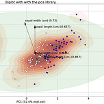
Image created by the PCA library. image by the author.

Principal Component Analysis is the most well-known technique for (big) data analysis. However, interpretation of the variance in the low-dimensional space can remain challenging. Understanding the loadings and interpreting the biplot is a must-know part for anyone who uses PCA. Here I will explain i) how to interpret the loadings for in-depth insights to (visually) explain the variance in your data, ii) how to select the most informative features, iii) how to create insightful plots, and finally how to detect outliers. The theoretical background will be backed by a practical hands-on guide for getting the most out of your data with pca.

---

Introduction

At the end of this blog, you can (visually) explain the variance in your data, select the most informative features, and create insightful plots. We will go through the following topics:

• Feature Selection vs. Extraction.

• Dimension reduction using PCA.

• Explained variance, and the scree plot.

• Loadings and the Biplot.

• Extracting the most informative features.

• Outlier detection.

---

Gentle introduction to PCA.

The main purpose of PCA is to reduce dimensionality in datasets by minimizing information loss. In general, there are two manners to reduce dimensionality: Feature Selection and Feature Extraction. The latter is used, among others, in PCA where a new set of dimensions or latent variables are constructed based on a (linear) combination of the original features. In the case of feature selection, a subset of features is selected that should be informative for the task ahead. No matter what technique you choose, reducing dimensionality is an important step for several reasons such as reducing complexity, improving run time, determining feature importance, visualizing class information, and last but not least preventing the curse of dimensionality. This means that, for a given sample size, and above a certain number of features the classifier will degrade in performance rather than improve (Figure 1). In most cases, a lower-dimensional space results in more accurate mapping and compensates for the “loss” of information.

In the next section, I will explain how to choose between feature selection and feature extraction techniques because there are reasons to choose between one or another.

Figure 1. The performance of (classifications) models as a function of dimensionality. (image by the author)

Feature selection.

Feature selection is necessary for several situations; 1. In case the features are not numeric (e.g., strings). 2. In case you need to extract meaningful features. 3. To keep measurements intact (a transformation would make a linear combination of measurements and the unit to be lost). A disadvantage is that feature selection procedures do require a search strategy and/or objective function to evaluate and select the potential candidates. As an example, it may require a supervised approach with class information to perform a statistical test or a cross-validation approach to select the most informative features. Nevertheless, feature selection can also be done without class information, such as by selecting the top N features on the variance (higher is better).

Figure 2. Schematic overview of the Feature Selection procedure. (image by the author)

Feature extraction.

Feature extraction approaches can reduce the number of dimensions and at the same time minimize the loss of information. To do this, we need a transformation function; y=f(x). In the case of PCA, the transformation is limited to a linear function which we can rewrite as a set of weights that make up the transformation step; y=Wx, where W are the weights, x are the input features, and y is the final transformed feature space. See below a schematic overview to demonstrate the transformation step together with the mathematical steps.

Figure 3. Schematic overview of the Feature Extraction procedure that linearly transforms the input data in the form y=Wx. (image by the author)

A linear transformation with PCA has also some disadvantages. It will make features less interpretable, and sometimes even useless for follow-up in certain use-cases. As an example, if potential cancer-related genes were discovered using a feature extraction technique, it may describe that the gene was partially involved together with other genes. A follow-up in the laboratory would not make sense, e.g., to partially knock out/activate genes.

---

How are dimensions reduced in PCA?

We can break down PCA into roughly four parts, which I will describe illustratively.

Part 1. Center data around the origin.

The first part is computing the average of the data (illustrated in Figure 4) which can be done in four smaller steps. First by computing the average per feature (1 and 2), and then the center (3). We can now shift the data so that it is centered around the origin(4). Note that this transformation step does not change the relative distance between the points but only centers the data around the origin.

Figure 4: Center data around zero. (image by the author)

Part 2. Fit the line through origin and data points.

The next part is to fit a line through the origin and the data points (or samples). This can be done by 1. drawing a random line through the origin, 2. projecting the samples on the line orthogonally, and then 3. rotating until the best fit is found by minimizing the distances. However, it is more practical to maximize the distances from the projected data points to the origin which will lead to the same results. The fit is computed using the sum of squared distances (SS) as it will eliminate the orientation of the data points surrounding the line. At this point (Figure 5), we fitted a line in the direction with the maximum variance.

Figure 5: Finding the best fit. Start with a random line (top) and rotate until it fits the data best by minimizing the distances from the data points to the line (bottom). (image by the author)

Part 3. Computing the Principal Components and the loadings.